Learning Invariant Sets from Failure
Safety-critical control systems require the state to remain within a prescribed set of admissible states at all times. We seek the invariant set and the control inputs that ensure invariance when the system dynamics are unknown.

The control problem
Consider the discrete-time controlled nonlinear time-invariant dynamical system
Here, x(k) ∈ ℝnx is the state and u(k) ∈ ℝnu is the control input. The mapping f : ℝnx × ℝnu → ℝnx is Lipschitz continuous with f(0, 0) = 0. The state is constrained to a compact set X containing the origin in its interior, and the input is constrained to a compact set U(x), with 0 ∈ U(0).
We wish to choose inputs that achieve a control objective while satisfying these constraints indefinitely. In model predictive control (MPC), we minimize a cost over a finite prediction horizon, apply the first optimal input, and solve again at the next observed state. The question is whether repeatedly solving a finite-horizon problem is enough to keep the system safe.
An illustrative application: drone motion
For simplicity, we illustrate this problem using the constrained double integrator from our numerical example. We interpret x1 as displacement from a reference height, x2 as vertical velocity, and u as the input:
|x1| ≤ 15, |x2| ≤ 10, |u| ≤ 5.
The drone is a schematic visualization of this discrete-time model. We use it to examine complete trajectories under MPC, first with exact dynamics and then with model mismatch. The invariant-set definitions that follow apply to the general nonlinear system (1).
From failing trajectories to invariant constraints
We choose a quadratic cost to regulate the example system to the origin. Play each case to follow the drone, its position over time, and its state-space trajectory.
N = 2, Q = I, R = 100, Vf(x) = x⊤x, x(0) = (−12, 7).
The dynamics and constraints are those of our double-integrator experiment. These controller settings define the additional MPC example below.
The MPC optimization problem
The variables xi|k and ui|k denote predictions made at time k.
The first and third cases continue until a state constraint is violated. The second and fourth show the corresponding remedies. All four start from the same state with the same cost, horizon, and physical constraints.
The moving drone and position trace show the full flight. The linked state-space plot shows the actual trajectory and the current MPC prediction. When MPC becomes infeasible, we apply maximum braking until the first constraint violation; the red cross marks that event. Playback stops at failure. In the safe cases, we show 20 MPC steps. Motion between discrete states is interpolated for display.
With exact dynamics and an initially feasible problem, an invariant terminal set provides an admissible continuation at every step.[1] Under model mismatch, we must also account for uncertainty in the transitions. Robust MPC imposes conditions that hold for a specified uncertainty set.[2]
The robust remedy used in the animation
We compute a robust control invariant set C for fα(x, u) = [x1 + αx2, x2 + u]⊤, with α ∈ [0.8, 1.2]. We use α = 0.8 for the nominal MPC prediction, impose xN|k ∈ C, and require the applied input to satisfy
The same input must keep every possible next state in C. This condition admits a feasible continuation from every state in C. The animation lets us vary the actual dynamics within the uncertainty interval.
The cost of requiring safety for every possible model
The robust remedy preserves safety, but it can exclude states that are invariant for the actual dynamics. The state (0, 9) lies in the true MCI and outside the robust set: under α = 1, braking keeps the drone within constraints, whereas under α = 1.2, even maximum braking reaches x1 = 15.6.
Rose: the MCI for the actual dynamics, α = 1. Blue: the robust invariant set for α ∈ [0.8, 1.2]. The marked state (0, 9) is removed by the robust requirement.
Same invariant state, different inputs
Must we discard the state (0, 9)? For the actual dynamics, the answer is no. The state admits an input that preserves safety, even though another admissible input leads to failure.
Preserving first input: u = −5
Both trajectories start at x(0) = (0, 9) ∈ X∞. The solid arrow applies the chosen first input; the dashed continuation then brakes toward zero velocity using admissible inputs. Rose is the true MCI. Green preserves invariance; red leaves it. Change the first input to see that safety depends on the input chosen at this same state.
The MCI set only characterizes where the system can remain safe but not which inputs at each state ensure invariance. In this example, we can retain the initial state if we restrict the first input to [−5, −3.5], rather than excluding the state itself.
With known dynamics, we can check which admissible inputs keep the next state in the MCI. With an approximate model, that check can be wrong, as the MPC example shows. We therefore seek both the invariant set and the control inputs that ensure invariance at each state, using observed transitions in place of a known dynamics model.
To represent this information, we must retain the association between each state and its admissible invariance-preserving inputs. We first state the definitions in state space, then extend the representation to include the input.
MPC background
[1] Rawlings, Mayne, and Diehl, Model Predictive Control: Theory, Computation, and Design, Chapter 2.
[2] Bujarbaruah, Rosolia, Stürz, and Borrelli, A Simple Robust MPC for Linear Systems with Parametric and Additive Uncertainty.
Control invariance
Consider system (1) with state and input constraints X and U(x) for all x ∈ ℝnx. A set C ⊆ X is called control invariant if, for every x ∈ C, there exists u ∈ U(x) such that f(x, u) ∈ C.
A set X∞ ⊆ X is called the maximal control invariant set (MCI) if
- X∞ is control invariant, and
- if C ⊆ X is any control invariant set, then C ⊆ X∞.
A set C ⊆ X is safe if it is a control invariant set with respect to (1) and U(x) for all x ∈ C.
The MCI set can be computed via the one-step predecessor operator. For any set Ω ⊆ ℝnx, define
as the set of all states from which there exists an admissible input that steers the system into Ω in one step. The MCI set can be obtained as the fixed point of the recursive iteration
The predecessor recursion. Rose is the current set; the pale red wedges were removed at this iteration. Two passes suffice and Ω₂ = X∞. The removed wedges hold the states descending too fast to stop above the floor, or climbing too fast to stop below the ceiling.
Invariance-preserving inputs
The MCI set only characterizes where the system can remain safe but not which inputs at each state ensure invariance. The existential quantifier in (2) discards all control information during the recursion.
We now define the invariance-preserving input set.
Consider system (1) and a set C ⊆ ℝnx. The invariance-preserving input set of C under dynamics f is the set-valued map UfC : ℝnx → 2ℝnu defined by
For convenience, we write Uf∞(x) ≜ UfX∞(x).
Given an initial state x(0) ∈ X∞, a controller that selects u(k) from Uf∞(x(k)) ∩ U(x(k)) for all k ∈ ℤ+, ensures that x(k) remains in X∞.
In the next section, we show that both X∞ and Uf∞(x) ∩ U(x) can be obtained simultaneously by extending the computation of invariant sets to the joint state-control space.
The joint state-control space
We now return to the general nonlinear system (1). The definitions and invariant-set characterization below apply to this system. We continue to use the double integrator to visualize the sets.
Let z = [x⊤ u⊤]⊤ ∈ ℝnx + nu denote a state-control vector, and let Z ⊆ ℝnx + nu be a set in the joint state-control space. We now define the two operations that allow us to decompose Z into the state and control spaces, respectively.
The state projection of Z is the mapping Πx : 2ℝnx + nu → 2ℝnx and, for a given x ∈ Πx(Z), the x-section of Z is the mapping UZ : ℝnx → 2ℝnu, given by
Note that we do not use the control projection Πu(Z) since it would yield all control inputs in Z irrespective of the state. The x-section UZ(x) preserves the coupling between states and controls in Z. Using these operations and given the state and input constraint sets X and U(x) for all x ∈ X, we construct the joint constraint set in the state-control space
We now define the notion of state-control invariant sets.
Consider system (1) and the joint constraint set Z given above. A set C ⊆ Z is called state-control invariant if, for every z ∈ C, there exists u+ ∈ ℝnu such that [f(x, u)⊤ (u+)⊤]⊤ ∈ C.
A set Z∞ ⊆ Z is called the maximal state-control invariant set if
- Z∞ is state-control invariant, and
- if C ⊆ Z is any state-control invariant set, then C ⊆ Z∞.
Similarly to the state-space case, Z∞ can be computed using a predecessor operator in the joint state-control space. For any set Ω ⊆ ℝnx + nu, define
that is, the set of all state-control vectors for which the next state f(x, u) has a non-empty x-section, i.e., UΩ(f(x, u)) ≠ ∅. The MSCI is then obtained as the fixed point of the recursive iteration
At each step, Ωk+1 retains only those state-control vectors in Ωk for which an input exists that, when paired with the next state, lies within Ωk. State-control vectors that lack such an input are discarded.
The MSCI Z∞ admits the following properties:
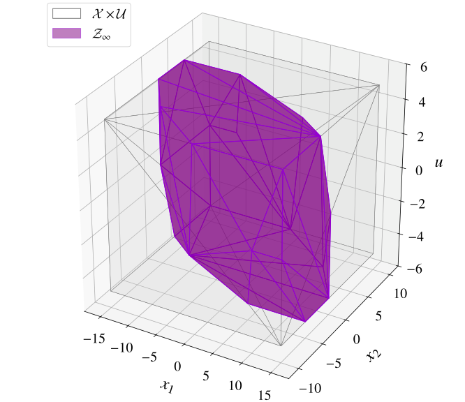
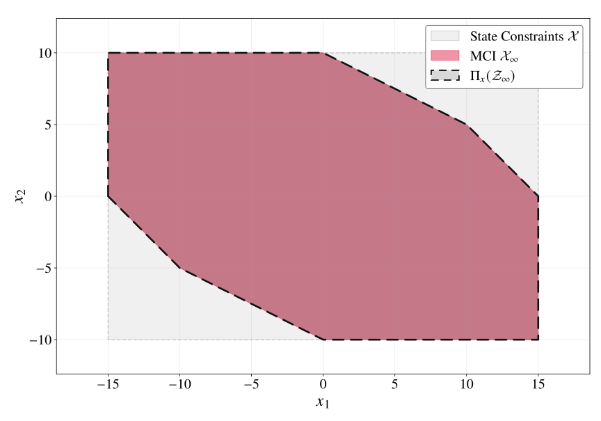
The MSCI set Z∞ is purple. Its state projection lies on the bottom plane, and the orange segment is the x-section at the selected state. Rotate the set or change the state to inspect how the admissible input interval varies.
From failures to halfspaces
We now specialize to deterministic LTI systems, f(x, u) = Ax + Bu, with polytopic constraints, and develop the failure-aware iterative learning (FAIL) algorithm.
At iteration ℓ, we write the current projected set as Xℓ−1 = {x : Hprojℓ−1x ≤ gprojℓ−1}. For linear dynamics, the predecessor is
The jth constraint of the projected set induces a predecessor halfspace with normal
Examining which constraints defined by Xℓ−1 were violated allows us to identify which predecessor constraints were violated and their corresponding (gprojℓ−1)j without knowing the dynamics.
A learning iteration can recover several halfspaces from the same failing trajectory. After each update, we check the stored trajectory against the updated set and continue learning until no new failures are identified. Below, we examine the regression for one halfspace at a time.
Next, we learn aj★ without knowing the dynamics. The z-space normal aj★ satisfies
for every time step t along any trajectory of (1). The left-hand side involves the unknown aj★, while the right-hand side is computed using (Hprojℓ−1)j and x(t+1). Hence, learning aj★ is a linear regression with z(t) being the regressor in ℝnx + nu, aj★ being the parameter to estimate, and (Hprojℓ−1)jx(t+1) being a measurement.
Let p ≜ nx + nu. To learn aj★, we require p linearly independent state-control samples. We form a window of p samples from available trajectory data
where t1, …, tp are time indices drawn from the failing trajectory or from other available trajectories. For these deterministic LTI dynamics, s = Z aj★ holds. If rank(Z) = p, the estimate of the normal vector âj is given by
Why three measurements?
The normal has three unknown components. Each observed transition supplies one equation: the state-control pair z(ti) forms a row of Z; the corresponding entry of s is (Hprojℓ−1)jx(ti+1). Three independent rows determine the normal. Repeating a row adds no independent information.
The figure shows one learned halfspace at a time. The final failing trajectory generates three halfspaces. The trajectory leaves the current projected set at the red-ringed next state. The orange facet supplies the known offset. Three independent transitions determine the three components of the predecessor normal. Open Why three measurements? to inspect the equations and the effect of dependent data.
Fit the halfspace yourself
Adjust the three components of âj to fit the observed transitions. The normal sets the orientation of the boundary; the offset translates it. The plots show which pairs your halfspace retains and removes.
Fit the normal: satisfy (8) for each observed transition, then check that the cut excludes the failure and preserves the MSCI reference.
The cut in state-control space
Blue: retained pairs. Red: MSCI region wrongly removed. The arrow shows the normal.
The x₁–x₂ projection
Blue: states with a retained input. Red: invariant states with no retained input.
Observed transitions and the regression in (8)
| Sample | x(ti) | u(ti) | x(ti+1) | (Hprojℓ−1)jx(ti+1) | âj⊤z(ti) | Difference |
|---|
We compare the two sides of (8): âj⊤z(ti) − (Hprojℓ−1)jx(ti+1). The offset does not enter this regression. These values are computed from the displayed simulated double-integrator trajectories; values are rounded for display.
Your candidate set is Pℓ−1 ∩ {z : âj⊤z ≤ (gprojℓ−1)j}. The right plot projects this set onto x₁–x₂. A cut can remove MSCI pairs while leaving every invariant state in this projection; red appears on the right only where no input remains. The cross marks the observed failure and its state. The dashed references are used only for this exercise; FAIL does not require them.
Each regression identifies p coefficients for one violated facet. Identifying (A, B) would require nxp coefficients before computing the predecessor sets.
The algorithm
Using the state projection and x-section of Pℓ, the state and input constraints at iteration ℓ are
The x-section Uℓ(x) is the algorithm's current estimate of the admissible invariance-preserving inputs at state x ∈ Xℓ.
At iteration ℓ, a one-step failing state-input vector zℓ = [(xℓ)⊤ (uℓ)⊤]⊤, with xℓ ∈ Xℓ−1 and uℓ ∈ Uℓ−1(xℓ), satisfies
Our goal is to exclude such states and inputs from the learned polytope. For each recovered halfspace, we apply the update
Each recovered halfspace contains Z∞ and excludes the observed failing pair. Thus, Z∞ ⊆ Pℓ ⊆ Pℓ−1: the iterates are decreasing outer approximations of the MSCI.
A learning iteration can generate more than one halfspace. The visualization advances through individual halfspace updates: trajectory 3 produces two halfspaces, and the final failing trajectory, trajectory 6, produces three. Trajectory 4 remains within the current set and produces none.
State projections (left) and joint sets (right). The learned set is blue; the reference boundary is black and dashed. Learn the next halfspace to inspect each update. This browser run uses six trajectories, five of which fail, to produce eight cuts, and P8 = Z∞ to numerical tolerance.
What the sections are for
At convergence, the section UL(x) contains exactly the admissible invariance-preserving inputs. Starting in the learned state projection and choosing an input from this section at every step keeps the trajectory within constraints.
The first state coordinate x₁ (left) and state-space trajectories (right). Each vehicle samples a new input at every step. Sampling from UL(x) preserves invariance. Switching to the original input set U(x) = [−5, 5] allows violations. A vehicle turns red when it leaves the learned MCI set and then applies maximum braking.
Numerical results
We now validate FAIL using constant-input and random admissible controllers to generate failing trajectories. The interactive figures simulate the same dynamics and compute their displayed values from the double-integrator dynamics.
We validate FAIL on the double-integrator example, with nx = 2, nu = 1, and p = 3. The bounds |x1| ≤ 15, |x2| ≤ 10, and |u| ≤ 5 define an initial polytope P0 with six constraints. FAIL does not know (A, B); we use these matrices only to simulate the system and compute the reference invariant sets.
Generating failing trajectories
We first apply the constant-input controllers u(k) ≡ −5 and u(k) ≡ 5 from x0 = [0, 0]⊤. We then sample initial states from Πx(Pℓ) and inputs uniformly from Uℓ(x(k)). Each trajectory runs for up to T = 15 steps and terminates when the state first leaves the current projected set.
Learning the MSCI
From six failing trajectories, we learn eight predecessor halfspaces in eight iterations. Together with the six initial constraints, these recover all 14 halfspaces of Z∞. At every iteration, we verify Z∞ ⊆ Pℓ and that the learned halfspace matches an MSCI constraint within a numerical tolerance of 10−3. At termination, P8 and Z∞ have Hausdorff distance zero, as do Πx(P8) and X∞.
| Method | Final constraints | Iterations | Time |
|---|---|---|---|
| MCI predecessor recursion | 8 | 2 | 0.19 s |
| MSCI predecessor recursion | 14 | 3 | 0.26 s |
| FAIL: learning the eight halfspaces | 14 | 8 | 0.0353 s |
We ran these experiments on a laptop with an Intel i9-11980HK CPU and an NVIDIA RTX 3080 GPU. The times above are from this experiment, not timings of the interactive figures.
At each iteration, we test up to 1,200 trajectories using the random admissible controller. At L = 8, none of the 1,200 trajectories leaves Πx(P8). The learned sections satisfy U8(x) = Uf∞(x) ∩ U(x), giving the admissible inputs that preserve invariance.
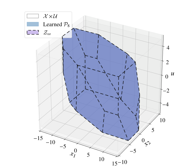
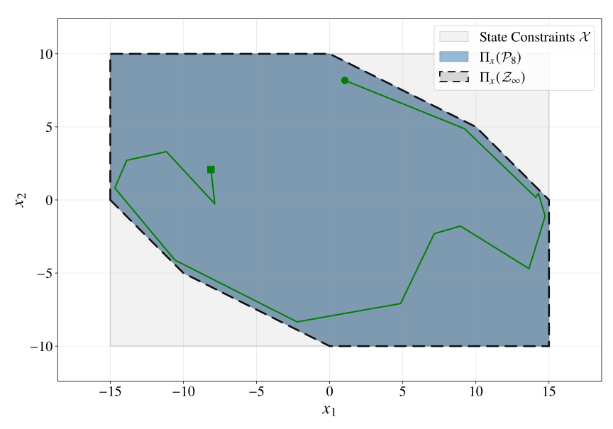
View the 1,200 non-failing trajectories
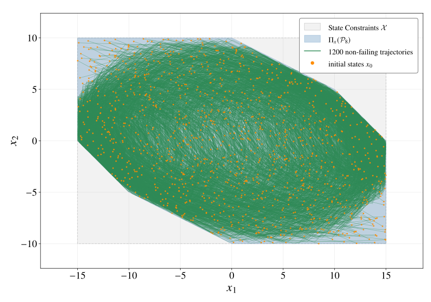
We generate 1,200 trajectories using the random admissible controller at L = 8. None leaves Πₓ(P₈). We also compare P₈ directly with Z∞ and obtain a Hausdorff distance of zero.
Future Work
Future research will focus on extending the framework to LTI systems with Gaussian noise.
Contributors
Ahmad Amine, Nick-Marios T. Kokolakis, Ugo Rosolia, Truong X. Nghiem, and Rahul Mangharam.
Citation
BibTeX
@inproceedings{amine2026failure,
  title={Failure-Aware Iterative Learning of State-Control Invariant Sets},
  author={Amine, Ahmad and Kokolakis, Nick-Marios T. and Rosolia, Ugo and Nghiem, Truong X. and Mangharam, Rahul},
  year={2026},
  booktitle={2026 IEEE 65th Conference on Decision and Control (CDC)},
  note={Accepted},
  eprint={2604.06776},
  archivePrefix={arXiv},
  primaryClass={eess.SY},
  url={https://arxiv.org/abs/2604.06776}
}
MLA
Amine, Ahmad, et al. “Failure-Aware Iterative Learning of State-Control Invariant Sets.” 2026 IEEE 65th Conference on Decision and Control (CDC), accepted, 2026.